Behavior Cloning Foundations

Behavior cloningbehavior cloningTraining a policy by supervised learning on expert demonstrations: each recorded observation is an input, the action the expert took at that moment is the label, and the fitted mapping from state to action is the policy. The recipe predates deep learning; ALVINN (1988) used camera and laser-range inputs and trained on simulated road images before NAVLAB tests, and the same approach, scaled to modern networks and datasets, still underlies most learned manipulation policies. Its known failure mode in closed loop is covariate shift. is the oldest way to make a robot imitate a person: record what an expert did, treat each observation as an input and the expert's action as the label, and fit a policy $\pi(a \mid s)$ by supervised learning. The idea predates deep learning. ALVINN (1988) used a three-layer back-propagation network with camera and laser-range inputs. It was trained on simulated road images and tested on NAVLAB, a modified Chevy van; training on real images while a human drives was proposed future work, not the reported training procedure Pomerleau 1988↓ALVINN: An Autonomous Land Vehicle in a Neural NetworkDean A. Pomerleau, Advances in Neural Information Processing Systems 1, 1988.

The appeal is obvious: no reward function to design, no exploration to manage, just regression onto demonstrations. The failure mode is equally specific, and nearly every architectural innovation in learned manipulation since 2023 is a partial answer to it. Supervised learning assumes that test inputs come from the same distribution as training inputs. A robot running in closed loop violates that assumption with its own actions.

Watch the error compound

This deterministic toy illustrates persistent drift, not a source benchmark or a task-cost theorem. Its error slider sets an additive error magnitude, not a measured failure probability. Per-timestep mode adds an error at every step; chunked mode adds one every 25 steps. The DAgger-labelled toggle removes 75% of the current deviation every 20 steps. These are illustration rules, not implementations or measured effects of ACT or DAgger. The readout sums absolute deviation; the dashed curves are reference scalings, not bounds on that sum.

Covariate shift, stated precisely

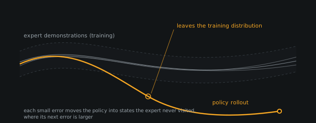
Training data is drawn from the expert's state distribution $d_{\pi^*}$. At deployment the robot visits its own distribution $d_\pi$, and the two diverge the moment the policy makes its first mistake. A small error moves the robot into a state slightly outside the demonstrations; from that unfamiliar state the policy is more likely to err again; each error pushes it further out. Ross, Gordon, and Bagnell made this precise: a policy with per-step error $\varepsilon$ on the expert distribution can incur total cost growing quadratically in the episode length $T$, and they gave a matching lower bound showing the quadratic term is unavoidable under i.i.d. training Ross 2011↓A Reduction of Imitation Learning and Structured Prediction to No-Regret Online LearningStéphane Ross, Geoffrey J. Gordon, J. Andrew Bagnell, AISTATS 2011.

For a task cost bounded in $[0,1]$ and a surrogate loss that upper-bounds imitation 0-1 loss, the two relevant statements are:

The first uses error $\varepsilon$ on the expert distribution. The second is DAgger’s conditional, infinite-sample Theorem 3.2: after $N=\tilde{O}(uT)$ iterations there exists a policy $\hat{\pi}$ in the learned sequence satisfying the bound. Here $\varepsilon_N$ is the true loss of the best policy in hindsight across the collected mixed-policy state distributions, not the expert-distribution error above. The factor $u$ bounds the increase in expert cost-to-go after one action. Linear-in-$T$ excess cost requires $u$ independent of $T$; in the worst case $u$ can be $O(T)$. The loss and mixing assumptions are stated in the DAggerDAggerDataset Aggregation, the iterative fix for behavior cloning's distribution mismatch: roll out the current policy, have the expert label the states the policy actually visits, add those labeled states to the training set, and retrain. Ross, Gordon, and Bagnell framed the procedure as a reduction of imitation learning to no-regret online learning, whose task-cost guarantee is existential over the learned sequence and requires learning and expert-mixing assumptions. Linear excess-cost scaling also requires the expert recovery-cost factor u to be independent of the horizon; u can be O(T) in the worst case. section below Ross 2011↓A Reduction of Imitation Learning and Structured Prediction to No-Regret Online LearningStéphane Ross, Geoffrey J. Gordon, J. Andrew Bagnell, AISTATS 2011. Physical Intelligence restated the same point in operational terms in 2025: it is relatively easy to get a learned policy to succeed at a task some of the time, and much harder to make it succeed reliably Amin 2025↓π*0.6: a VLA that Learns from ExperienceAli Amin, Raichelle Aniceto, Ashwin Balakrishna et al., 2025.

Original schematic

Diagram: Robot Wiki contributors / Robot Wiki (original diagram). Licence: CC BY 4.0.

Fitting demonstrations is hard before deployment even starts

Compounding errorcompounding errorThe accumulation of small per-step mistakes over the course of a sequential task: each error carries the robot into a state slightly outside its training data, where the next error is more likely, so total deviation grows faster than the per-step error rate. Ross, Gordon, and Bagnell bounded the effect for imitation learning with total cost quadratic in episode length, and action chunking attacks the same effect from the other side by shrinking the number of sequential decisions in an episode. is the deployment problem. Three training-side problems compound it:

Multimodality. Human demonstrations can contain several valid action strategies. Diffusion Policydiffusion policyA policy that produces actions through a conditional denoising diffusion process over a whole action sequence instead of regressing a single action directly. Introduced by Chi et al. in 2023, it represents multimodal demonstrations faithfully rather than averaging their modes, and it executes only the first few steps of each predicted sequence before observing again and replanning. models multimodal action distributions: in its Push-T example it learns both modes, left-going and right-going, and commits to one mode within a rollout Chi 2023↓Diffusion Policy: Visuomotor Policy Learning via Action DiffusionCheng Chi, Zhenjia Xu, Siyuan Feng et al., 2023.

Temporally correlated confounders. Demonstrations contain pauses and idle segments that are unpredictable from a single Markovian state. A single-step policy cannot tell "waiting" from "acting," and both ACT and Diffusion Policy document robots freezing in place because of it Zhao 2023↓Learning Fine-Grained Bimanual Manipulation with Low-Cost HardwareTony Z. Zhao, Vikash Kumar, Sergey Levine et al., RSS 2023 Chi 2023↓Diffusion Policy: Visuomotor Policy Learning via Action DiffusionCheng Chi, Zhenjia Xu, Siyuan Feng et al., 2023. The fix is temporal context, not a larger backbone.

The demonstration ceiling. Behavior cloning can at best match the demonstrator. If the teleoperator is slow, cautious, or inconsistent, the policy inherits all of it, and the covariate-shiftcovariate shiftIn imitation learning, the mismatch between the state distribution in the training demonstrations and the distribution the learned policy visits at deployment. The policy's own errors carry it into states the demonstrations never covered, where it is likelier to err again, so mistakes compound: Ross, Gordon, and Bagnell showed that a behavior-cloned policy with per-step error ε can incur total cost growing quadratically in episode length, and that no i.i.d.-trained policy can guarantee better. analysis above means it will usually do worse.

DAgger: relabel the states you actually visit

DAgger (Dataset Aggregation) attacks the quadratic bound directly Ross 2011↓A Reduction of Imitation Learning and Structured Prediction to No-Regret Online LearningStéphane Ross, Geoffrey J. Gordon, J. Andrew Bagnell, AISTATS 2011. The loop:

DAgger reduces imitation learningimitation learningLearning a policy from expert demonstrations rather than from a reward signal: the expert's recorded state-action pairs become a supervised training set, and the fitted mapping from observed state to action is the policy. Pomerleau's ALVINN (1988) instead trained on simulated road images before steering NAVLAB, and the recipe still underlies most learned manipulation. Its structural weakness is that the training distribution comes from the expert while deployment visits the states the learner itself induces, the mismatch DAgger was designed to repair. to no-regret online learning. Its guarantee is existential over the learned sequence, not a promise that every iterate improves. Theorem 3.2 assumes a bounded, strongly convex surrogate loss that upper-bounds imitation 0-1 loss, with expert mixing $\beta_i \leq (1-\alpha)^{i-1}$ for a constant $\alpha$ independent of $T$. It uses the true best-policy-in-hindsight loss

The analysis allows selection of the sequence policy with the lowest true loss under its own state distribution, or uniformly choosing a sequence policy once for an entire episode. Algorithm 3.1 returns the best policy on validation; it does not guarantee that the last iterate is best. Finite-sample Theorem 3.4 instead uses empirical training loss $\hat{\varepsilon}_N$: with $m=O(1)$ trajectories per iteration and $N=O(u^2T^2\log(1/\delta))$, the analogous bound holds for some sequence policy with probability at least $\left(1-\delta\right)$. On-policy coverage alone neither makes $u$ constant nor guarantees linear task cost Ross 2011↓A Reduction of Imitation Learning and Structured Prediction to No-Regret Online LearningStéphane Ross, Geoffrey J. Gordon, J. Andrew Bagnell, AISTATS 2011.

The catch is the expert. Classic DAgger needs a supervisor who can look at an arbitrary mid-failure robot state and name the correct action, which is unnatural and slow for a human teleoperator. HG-DAgger (the retained arXiv v2 text) gives the human expert uninterrupted control when they judge intervention necessary. The expert guides the system back to a safe, stable region; action labels are collected during these recovery trajectories, and the expert manually returns control to the novice Kelly 2019↓HG-DAgger: Interactive Imitation Learning with Human ExpertsMichael Kelly, Chelsea Sidrane, Katherine Driggs-Campbell et al., arXiv v2 (11 March 2019). Fourteen years later, the same pattern shows up as the "coaching" stage of Physical Intelligence's Recap, where human corrections on visited states fine-tune a vision-language-action policy Amin 2025↓π*0.6: a VLA that Learns from ExperienceAli Amin, Raichelle Aniceto, Ashwin Balakrishna et al., 2025.

Where this leads

These results separate three questions: can a policy fit demonstrations, will it visit states covered by training, and can the expert recover after a mistake? Action chunking addresses temporal action structure. Diffusion Policy represents multiple action modes. DAgger collects expert labels on visited states. None of those mechanisms alone establishes an unconditional long-horizon task-cost guarantee.

References

Dean A. Pomerleau, Advances in Neural Information Processing Systems 1, 1988.
https://proceedings.neurips.cc/paper/1988/hash/812b4ba287f5ee0bc9d43bbf5bbe87fb-Abstract.html
Stéphane Ross, Geoffrey J. Gordon, J. Andrew Bagnell, AISTATS 2011.
https://arxiv.org/abs/1011.0686
Michael Kelly, Chelsea Sidrane, Katherine Driggs-Campbell, Mykel J. Kochenderfer, arXiv v2 (11 March 2019).
https://arxiv.org/abs/1810.02890
Ali Amin, Raichelle Aniceto, Ashwin Balakrishna, Kevin Black, Ken Conley, Grace Connors, James Darpinian, Karan Dhabalia, and 47 more, 2025.
https://www.pi.website/blog/pistar06
Tony Z. Zhao, Vikash Kumar, Sergey Levine, Chelsea Finn, RSS 2023.
https://arxiv.org/abs/2304.13705
Cheng Chi, Zhenjia Xu, Siyuan Feng, Eric Cousineau, Yilun Du, Benjamin Burchfiel, Russ Tedrake, Shuran Song, 2023.
https://arxiv.org/abs/2303.04137
Spot a factual error or missing qualification? Report a content correction.